
Anyone who’s driven over the crest of a hill and briefly lost sight of the road ahead — or felt that gentle “settling” sensation dropping into a dip — has experienced a vertical curve, whether they realized it or not. Vertical curve design for road grading is the part of roadway design that smooths out these transitions between different grades, and it’s governed by two interconnected ideas: K-values and sight distance.
Get these wrong, and you end up with a road that either feels harsh to drive on or, more seriously, hides oncoming hazards from drivers until it’s too late to react. This guide walks through what vertical curves are, how K-values work, how sight distance drives the whole design process, and how to actually calculate curve lengths for a grading project.
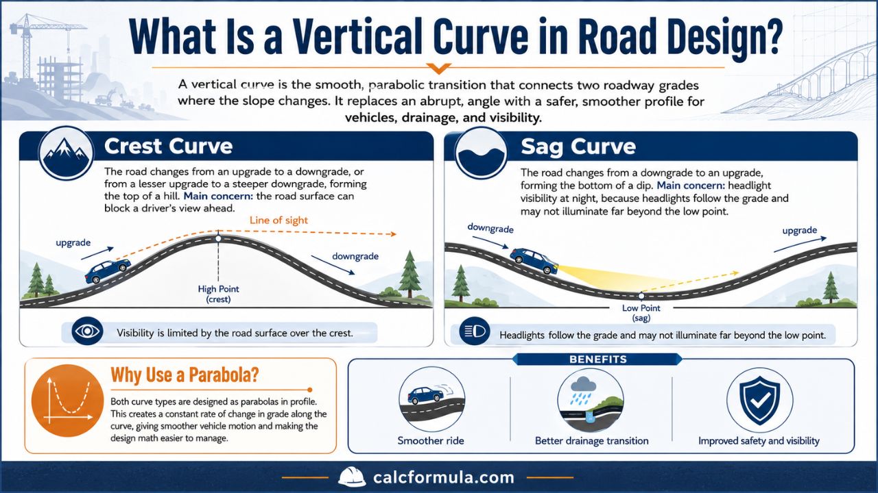
What Is a Vertical Curve in Road Design?
A vertical curve is the smooth, parabolic transition that connects two roadway grades (slopes) at a point where the grade changes. Without it, a road would have an abrupt angle wherever the slope shifts — uncomfortable for vehicles, hard on drainage, and dangerous because of how it affects visibility.
There are two basic types:
- Crest curves — the roadway goes from an upgrade to a downgrade (or a lesser upgrade to a steeper downgrade), forming the top of a hill. The main concern here is that the road surface itself can block a driver’s view of what’s ahead.
- Sag curves — the roadway goes from a downgrade to an upgrade, forming the bottom of a dip. The main concern here shifts to headlight visibility at night, since headlights point along the grade rather than illuminating the road beyond the low point.
Both curve types are designed as parabolas in profile, which gives a constant rate of change in grade along the curve — a property that makes the math much more manageable than it might look at first glance.
Grades, the Algebraic Difference (A), and Why It Matters
Before getting into K-values, it helps to nail down a couple of terms that show up throughout vertical curve design.
Grade (g) is the slope of the roadway, expressed as a percentage — rise over run, multiplied by 100. An upgrade is positive, a downgrade is negative.
Algebraic difference (A) is simply the difference between the two grades that meet at the point of vertical intersection (PVI):
A = g2 − g1
For a crest curve, this value works out negative (the road is curving downward relative to the incoming grade). For a sag curve, it’s positive. In practice, most designers work with the absolute value of A, since the formulas care about the magnitude of the grade change, not its direction.
If you’re working from survey data or a grading plan and need to confirm the actual percentage grades along a route before running any curve calculations, a Grade Slope Calculator is a fast way to convert rise-and-run measurements into the percentage grades you’ll plug into the vertical curve formulas.
What Is a K-Value in Vertical Curve Design?
This is the term that trips people up the most, mostly because it sounds more abstract than it actually is.
K-value is defined as the horizontal distance, in feet, required to achieve a 1% change in grade.
Mathematically:
K = L ÷ A
Where L is the length of the vertical curve and A is the algebraic difference in grades (as a percentage).
Rearranged, this gives you the formula most designers actually use day to day:
L = K × A
The key thing to understand is that K isn’t something you calculate from scratch for every project — it’s a design control value that comes from sight distance requirements based on the design speed of the road. Transportation agencies publish K-value tables (most based on the AASHTO “Green Book” methodology) that tell you the minimum K-value needed for a given design speed, separately for crest curves and sag curves, since the controlling criteria are different for each.
Once you know your design speed, you look up the appropriate K-value, multiply it by your algebraic difference in grades, and that gives you the minimum required curve length.
Sight Distance: The Real Driver Behind Vertical Curve Length
K-values aren’t arbitrary — they exist because of stopping sight distance (SSD), which is the distance a driver needs to see ahead in order to perceive a hazard, react, and bring the vehicle to a stop before reaching it. SSD itself is a function of design speed, driver reaction time, and braking distance, and it increases significantly as speed increases.
For crest curves, the limiting factor is geometric: the curve of the road surface itself creates a sightline obstruction. A driver’s eye height and the height of an object on the road (traditionally a low obstacle) determine how far the driver can see over the crest. The flatter and longer the curve, the farther a driver can see — which is why higher design speeds require larger K-values and longer curves.
For sag curves, daytime sight distance generally isn’t the issue, since the road ahead is visible. At night, however, the limiting factor becomes the headlight beam distance — how far ahead the headlights illuminate the roadway as the vehicle approaches and passes through the low point of the curve. A sag curve that’s too short causes the headlight beam to point into the pavement too close to the vehicle, leaving the road ahead in darkness.
This is also why crest and sag K-values for the same design speed are usually different numbers — they’re solving for two different visibility problems.
Minimum Curve Length Formulas
For most design situations, the relevant formulas (based on stopping sight distance, in U.S. customary units) are as follows.
Crest Curves
When the sight distance (S) is less than the curve length (L):
L = A × S² ÷ 2158
When the sight distance is greater than the curve length:
L = 2S − (2158 ÷ A)
(The constant 2158 comes from the standard assumed driver eye height of 3.5 feet and object height of 2.0 feet used in stopping sight distance calculations. Some agencies use slightly different assumed heights, which changes this constant — always check the standard your jurisdiction follows.)
Sag Curves
When the sight distance is less than the curve length:
L = A × S² ÷ (400 + 3.5S)
When the sight distance is greater than the curve length:
L = 2S − (400 + 3.5S) ÷ A
(This version is based on headlight sight distance, using a 2-degree upward headlight divergence angle, which is the most common basis for sag curve design.)
In nearly every practical case, designers don’t solve these formulas from raw inputs every time. Instead, they use the K-value tables (derived from these same formulas at standard design speeds) and apply L = K × A directly. The formulas above are mainly useful for checking non-standard situations or understanding where the K-value tables actually come from.
How K-Values Relate to Design Speed
K-value tables increase with design speed, which makes intuitive sense — faster roads need longer sight distances, which means longer curves for the same grade change. While exact published values vary slightly between AASHTO editions and individual state DOT standards, the general pattern looks something like this for stopping sight distance:
| Design Speed | Typical Crest K (approx.) | Typical Sag K (approx.) |
|---|---|---|
| 30 mph | ~19 | ~37 |
| 40 mph | ~44 | ~64 |
| 50 mph | ~84 | ~96 |
| 60 mph | ~151 | ~136 |
| 70 mph | ~247 | ~181 |
These numbers are illustrative of the general trend and the relationship between crest and sag values — for an actual design, always pull the current K-values from the AASHTO Green Book or your governing agency’s roadway design manual, since the exact figures used for permits and approvals need to match the standard your reviewing agency applies.
Step-by-Step: Designing a Vertical Curve
Here’s a practical sequence for working through a vertical curve design once you know the grades on either side of a PVI.
1. Establish the Design Speed
This comes from the functional classification of the road and is typically set early in the project, often by the governing transportation agency.
2. Determine the Incoming and Outgoing Grades
Pull g1 and g2 from the proposed profile. If you’re working from field data or a preliminary grading plan, a Grade Slope Calculator can help confirm these percentages from elevation and distance measurements before you move forward.
3. Calculate the Algebraic Difference (A)
Subtract: A = g2 − g1. Take the absolute value for use in the K-value formula, and note whether the result indicates a crest or sag curve.
4. Select the Appropriate K-Value
Using the design speed, look up the minimum K-value from the relevant table — crest or sag, depending on which type of curve you’re designing.
5. Calculate the Minimum Curve Length
Apply L = K × A to get the minimum required length. Many agencies also apply a separate minimum length rule independent of K-value (often something like “length should be at least three times the design speed in mph, expressed in feet”) to avoid curves that are mathematically adequate but uncomfortably short in the field.
6. Lay Out the Curve and Compute Elevations Along It
Once the curve length is set, the next step is computing elevations at regular stations along the curve — needed for grading plans, cut/fill calculations, and staking. A Vertical Curve Calculator handles this directly: enter your grades, curve length, and PVI station/elevation, and it returns the elevation at any point along the parabola, including the high or low point of the curve.
7. Verify Elevations Against the Existing Grading Plan
Before finalizing, cross-check the computed curve elevations against existing ground elevations and other site constraints — an Elevation Calculator Construction tool is useful here for quickly working through elevation differences across the site as you confirm the design fits within the available grading envelope.
Other Design Considerations Beyond the Minimum
Meeting the minimum K-value isn’t always the end of the story. A few other factors commonly come into play:
- Drainage on sag curves. Very flat sag curves can create drainage problems at the low point if the grade becomes too shallow for water to flow off the pavement effectively. Many agencies specify a minimum grade near the low point of a sag curve for this reason.
- Passing sight distance. On two-lane roads, crest curves on segments designated for passing zones may need to be designed for passing sight distance rather than just stopping sight distance — which requires significantly longer curves.
- Rider comfort. On sag curves especially, very short curve lengths combined with high speeds can create an uncomfortable vertical acceleration (“g-force”) for occupants, even if sight distance requirements are technically met. Some agencies apply a comfort-based minimum length as an additional check.
- Constructability. Extremely long curves driven by high design speeds can sometimes conflict with right-of-way limits or existing infrastructure, requiring a broader look at the overall vertical alignment rather than adjusting a single curve in isolation.
Common Mistakes in Vertical Curve Design
A handful of issues tend to come up repeatedly, even on otherwise well-designed projects:
- Using the wrong K-value table — applying a crest K-value to a sag curve (or vice versa), which can result in a curve that’s either unnecessarily long or critically short
- Forgetting the sign convention when calculating A, leading to confusion about whether a curve is a crest or sag condition
- Mixing up sight distance and curve length in the “S < L” vs. “S > L” cases, which use different formula forms
- Skipping the minimum length check that exists independent of the K-value formula, resulting in curves that are mathematically valid but feel abrupt to drivers
- Not verifying the final design against current AASHTO or agency-specific K-value tables, since published values have shifted somewhat between editions as design assumptions (like driver eye height) have been updated
Frequently Asked Questions
What does K-value mean in vertical curve design?
K-value represents the horizontal distance, in feet, needed to produce a 1% change in grade along a vertical curve. It’s used as a design control value: multiply the K-value for a given design speed by the algebraic difference in grades to get the minimum required curve length (L = K × A).
Why are crest and sag K-values different for the same design speed?
Crest curves are governed by daytime stopping sight distance, limited by the geometry of the road surface blocking a driver’s line of sight. Sag curves are typically governed by nighttime headlight sight distance, since the road ahead is otherwise visible during the day. These are different physical problems, so they produce different K-values even at the same design speed.
How do I calculate the length of a vertical curve?
Once you know the design speed, look up the appropriate K-value (crest or sag) from a standard table, calculate the algebraic difference in grades (A = g2 − g1), and multiply: L = K × A. This gives the minimum curve length based on sight distance.
What’s the difference between a crest curve and a sag curve?
A crest curve occurs where the roadway transitions from an upgrade to a downgrade, forming the top of a hill — the visibility concern is the road surface blocking the driver’s view. A sag curve occurs where the roadway transitions from a downgrade to an upgrade, forming a dip — the visibility concern shifts to headlight beam distance at night.
Final Thoughts
Vertical curve design for road grading boils down to a fairly compact set of ideas once the terminology is sorted out: a parabolic transition connects two grades, the algebraic difference between those grades drives the required curve length, and K-values translate sight distance requirements at a given design speed into a length you can actually apply. The hardest part usually isn’t the arithmetic — it’s making sure you’re using the right K-value table for the right curve type, and double-checking the result against current design standards before it goes into a grading plan.
Once the grades, algebraic difference, and K-value are sorted out, the remaining work — computing station elevations, checking the high or low point, and verifying the design against existing grades — is mostly a matter of careful, repeatable calculation.